Blog : Plotting Von Karman vortex street
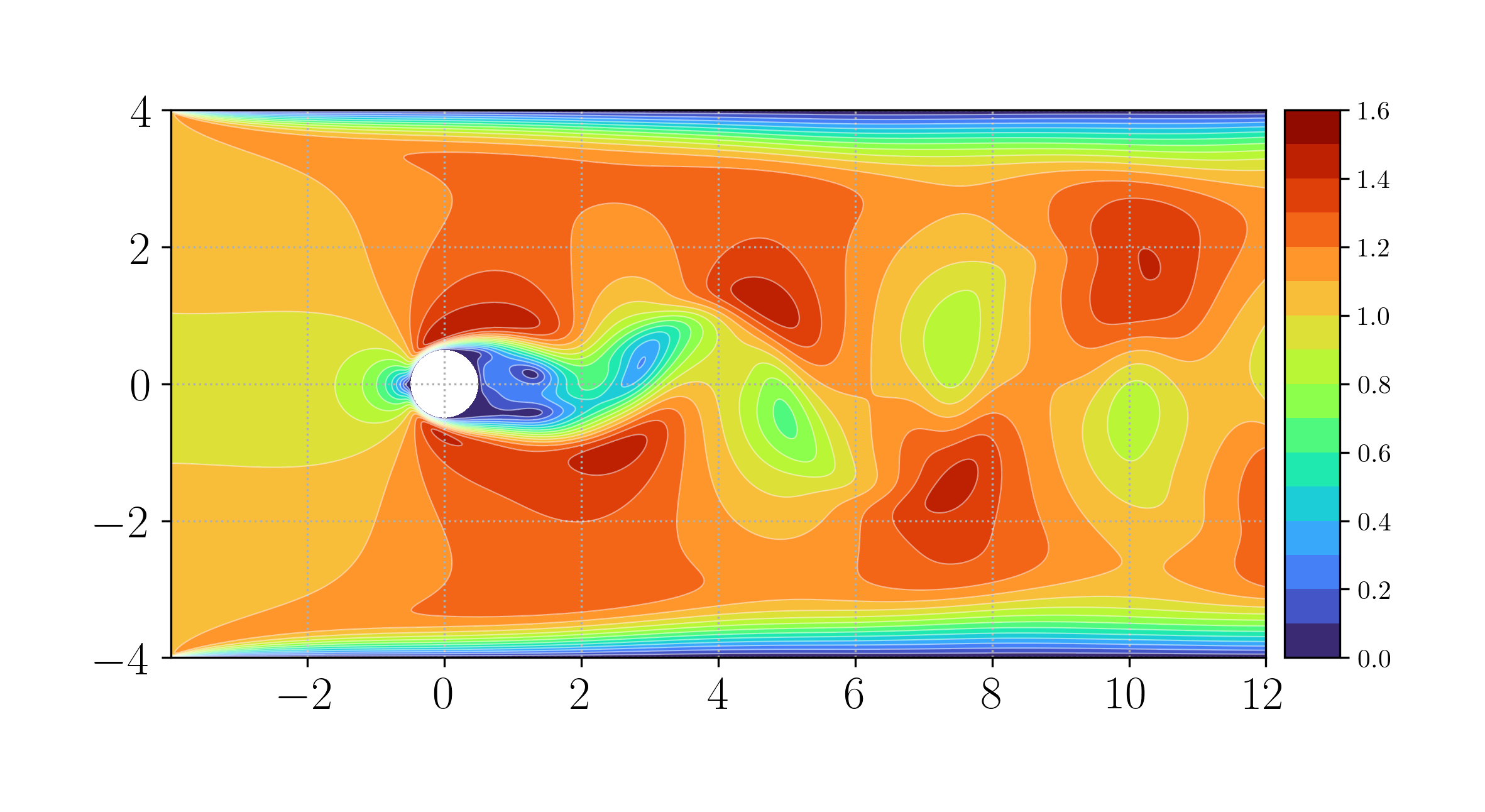
Let’s imagine we need velocity contour plots in vector format (SVG, PDF).
Usually, we use Matplotlib for this purpose. It includes tricontourf function,
which can even triangulate data. However, here we have a hole in the data (the
cylinder) that should not be triangulated. Therefore, we use VTK output from
cuttingPlane function object.
The plotting is split into data preparation and the plotting itself.
For data preparation, we use VTK Python module to read the data and triangulate
it for compatibility with the Matplotlib. Then we extract the vertices, velocity
values, and triangles, which are subsequently passed to the tricontourf function.
The Python code for the described procedure is shown below.
First, we import necessary modules:
#!/usr/bin/env python3

import vtk
from vtk.util import numpy_support

import numpy as np

import matplotlib.pyplot as plt
from mpl_toolkits.axes_grid1 import make_axes_locatable
First is VTK, which is used for reading and manipulating
function object output. Then we import Numpy for fast
array manipulations, and finally we import Matplotlib
for plotting. make_axes_locatable is needed for the color bar.
reader = vtk.vtkXMLPolyDataReader()

reader.SetFileName('postProcessing/surfacesf/200/centerPlane.vtp')
reader.Update()

data = reader.GetOutput()

triangle_filter = vtk.vtkTriangleFilter()
triangle_filter.SetInputData(data)
triangle_filter.Update()
data = triangle_filter.GetOutput()
Next, we read and triangulate the velocity data.
vtk_points = data.GetPoints().GetData()
points = numpy_support.vtk_to_numpy(vtk_points)
x = points[:, 0]
y = points[:, 1]

vtk_vectors = data.GetPointData().GetArray("U")

vtk_cells = data.GetPolys().GetData()
cells_raw = numpy_support.vtk_to_numpy(vtk_cells)
triangles = cells_raw.reshape(-1, 4)[:, 1:]

U = numpy_support.vtk_to_numpy(vtk_vectors)
magU = np.linalg.norm(U, axis=1)
Then we extract VTK file vertices, cell velocity values, triangles, and calculate the velocity magnitude.
fig, ax = plt.subplots(figsize=(8, 6))

contour_filled = ax.tricontourf(x, y, triangles, magU, levels=16, cmap="turbo")

ax.tricontour(
    x, y, triangles, magU, levels=16, colors="white", linewidths=0.5, alpha=0.5
)

plt.xticks(fontsize=18)
plt.yticks(fontsize=18)

divider = make_axes_locatable(ax)
cax = divider.append_axes("right", size="5%", pad=0.1)

cbar = fig.colorbar(contour_filled, cax=cax)
ax.set_aspect("equal")
Finally, we plot the data. Color bar adjustments were necessary to match the height of the plot.
for f in ["svg", "pdf", "eps", "png"]:
    plt.savefig("velocity.{}".format(f), dpi=300, bbox_inches="tight", pad_inches=0.5)
And finally we save the plot in the desired file formats. A high contour count in vector formats makes the files larger than PNG, but they can be zoomed without losing quality.