Blog : Simulating Von Karman vortex street

Motivation

Once upon a time, I simulated the von Karman vortex street; the mesh was generated with Gmsh, I played with different discretization schemes and residual controls, and plotted VTK post-processing output with Matplotlib. This time I have decided to create a benchmark case, which uses all new convenience features introduced in OpenFOAM since then.

Geometry & mesh

Geometry is a simple 2D straight rectangular channel 16D × 8D, where D is our cylinder diameter (see figure below). The cylinder is located 4D downstream of the inlet. This corresponds to the geometry in the article (https://onlinelibrary.wiley.com/doi/abs/10.1002/fld.1683), where we can also find the values of force coefficients. Though the purpose of these simulations is to show the capabilities of OpenFOAM dictionaries, having reference values is a nice addition.

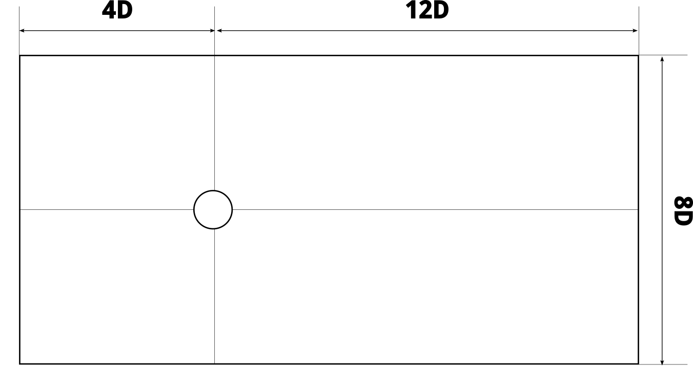
Meshing a cylinder in a channel

To mesh a geometry with the blockMesh utility, we first need to split it into hexahedral blocks. Then we put vertices of the blocks into the vertices list, put blocks in the blocks list, add curved edges description in the edges list, and finally put the mesh boundary patches in the boundary list.

Function entries in OpenFOAM dictionaries

Dictionaries in OpenFOAM use C-like syntax; as a consequence, there are function entries, which start with # to imitate the C preprocessor. The first function entry, which we will use in our case, is include, which simply includes the content of another dictionary in the place of the invocation. To simplify case management, we move all user-modifiable variables to a settings dictionary in the root folder of the case, which is then included with the #include "<case>/settings" entry.

In addition to the variable storage, we need to perform certain calculations (mesh density, number of cells in the graded zones, etc.). Earlier, OpenFOAM provided a calc entry for the purpose. It creates a C++ file with the expression, compiles it, and inserts the output of the code invocation in the dictionary. In modern versions, an eval entry evaluates expressions directly without compiling an external dynamic library.

And finally, there are conditional entries: if and ifeq. The first checks if the expression evaluates to true (in terms of OpenFOAM, so the expression can be yes or on). The second compares two expressions. In both cases, if the evaluation is true, the part after if is inserted in the dictionary; otherwise, the optional else part is used.

Settings dictionary

In the settings dictionary, we keep cylinder diameter, mesh cell sizes, and flow conditions. The first defines the geometry of the channel, the second defines the density of the mesh, and the last defines properties of the fluid. Since vortex shedding depends on the Reynolds number, we calculate fluid viscosity from cylinder diameter, the inlet velocity, and the Reynolds number.

We use a 2D mesh in the simulation, so we have a vertical size of the mesh (dz) and two average cell sizes: in the free flow zone (dx) and near the cylinder (dx_fine). To reduce the number of cells, we can use the mesh grading (grading).

blockMeshDict dictionary

Before writing the dictionary, we need to split our geometry into hexahedral blocks and define skeleton vertices, which are then used to construct the mesh.

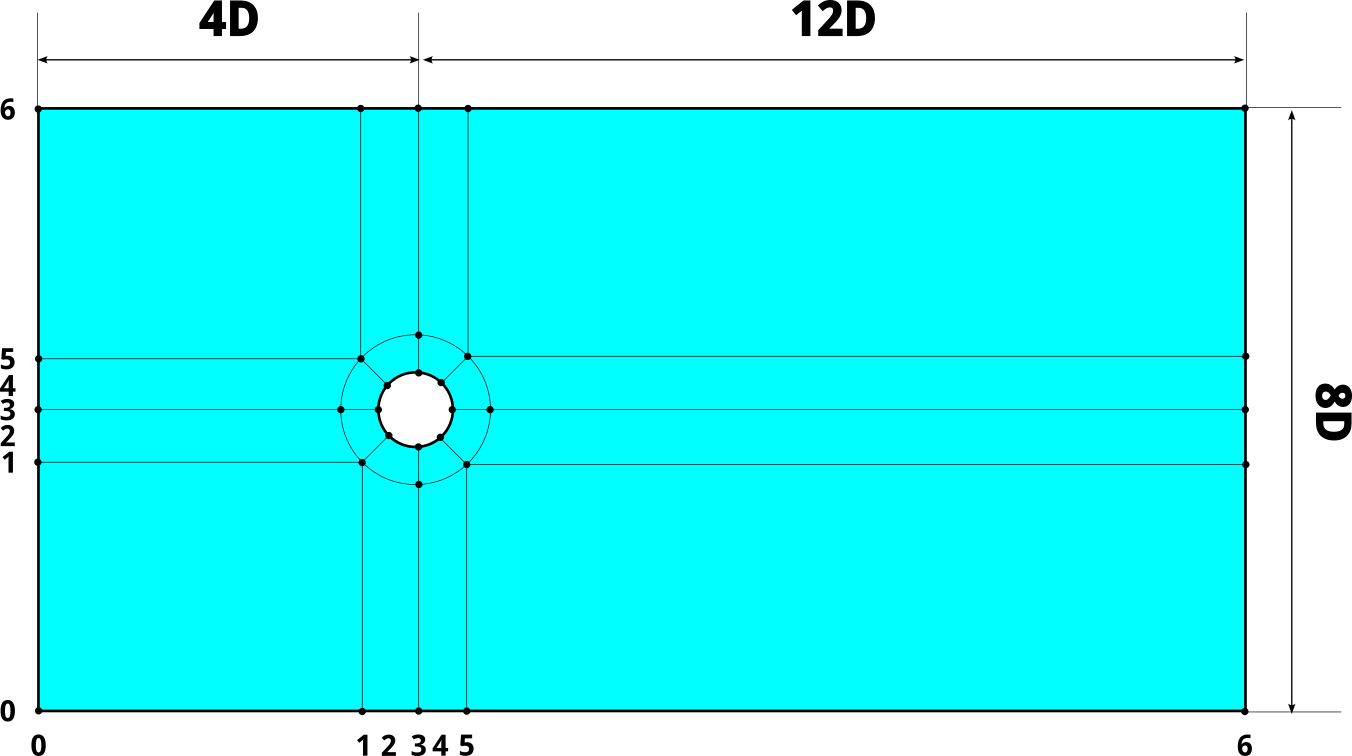
The mesh blocks scheme is shown in figure above. To have uniform normal cell size at the cylinder patch, we introduce additional vertices around it, so, in our mesh, we have 20 blocks: 4 near the inlet, 4 near the outlet, and 12 in the cylinder area.

The blockMeshDict starts with the inclusion of the settings dictionary, and then we calculate convenience variables using the eval function entry.

#include "<case>/settings"

R #eval "0.5*$D";

a #eval "$R/sqrt(2)";
b #eval "$D/sqrt(2)";
c #eval "4*$D";
d #eval "12*$D";


z0 -$dz;
z1  $dz;

Then mesh density and grading factors are calculated. Here, we use conditional entry #if and an analytical solution for the number of cells in the graded area. Since we have different grading directions in different areas, we calculate two grading factors, one for the mesh refinement and another for the mesh coarsening.

#if $grading

q #eval "$dx_fine/$dx";
p #eval "$dx/$dx_fine";

Ng #eval "ceil(log($q)/log(($b - $dx)/($b - $dx_fine)))";

#else

q 1;
p 1;

Ng #eval "ceil($b/$dx)";

#endif

Then we define the number of cells in different parts of the mesh; since we have 4 subdivisions in the X and Y directions, there are 4 values defined.

Nx1 #eval "ceil(($c - $b)/$dx)";
Nx2 $Ng;
Nx3 $Ng;
Nx4 #eval "ceil(($d - $b)/$dx)";


Ny1 #eval "ceil(($c - $b)/$dx)";
Ny2 $Ng;
Ny3 $Ng;
Ny4 #eval "ceil(($c - $b)/$dx)";

We need curved edges in our mesh: the edges of the cylinder and the edges of the blocks around the cylinder. In earlier OpenFOAM versions, defining edges required two endpoints and a third midpoint along the arc (defining the arc by three points). Now we can project a straight edge on the curved geometry. For this we first need to define the geometry, which is done in the geometry dictionary. There are two cylinders defined, the first one with the real cylinder geometry and the second, which is twice as large, for the “uniformization” blocks.

geometry
{
    cylinder1
    {
        type cylinder;
        point1 (0 0 -100);
        point2 (0 0 100);
        radius $R;
    }

    cylinder2
    {
        type cylinder;
        point1 (0 0 -100);
        point2 (0 0 100);
        radius $D;
    }
}

For the vertices definition, we use named vertices. In the earlier OpenFOAM versions, it was necessary to use vertex index in the block definition (starting with 0). This manual indexing approach is tedious and error-prone. So, for the vertices in this simulation, we use named vertices. And to simplify the mesh blocks description, we use mnemonics for the vertex names:

v<shift in the X direction><shift in the Y direction><shift in the Z direction>

Shift numbers correspond to the values on the scheme above. Utilization of the named vertices allows us to avoid tracking vertex index, and the shifts convention simplifies the construction of the blocks.

vertices
(
    name v000 (-$c -$c $z0)
    name v100 (-$b -$c $z0)
    name v300 (  0 -$c $z0)
    ...
);

Block description uses named vertices and precalculated variables (block densities, grading factors).

blocks
(
    hex (v000 v100 v110 v010 v001 v101 v111 v011) ($Nx1 $Ny1 1) simpleGrading ( 1  1 1)
    hex (v100 v300 v310 v110 v101 v301 v311 v111) ($Nx2 $Ny1 1) simpleGrading ($q  1 1)
    hex (v300 v500 v510 v310 v301 v501 v511 v311) ($Nx3 $Ny1 1) simpleGrading ($p  1 1)
    hex (v500 v600 v610 v510 v501 v601 v611 v511) ($Nx4 $Ny1 1) simpleGrading ( 1  1 1)
    ...
);

Curved edges of the mesh are described through the projection of the straight edges on the defined geometry.

edges
(
    project v110 v310 (cylinder2)
    project v310 v510 (cylinder2)
    project v510 v530 (cylinder2)
    project v530 v550 (cylinder2)
    project v550 v350 (cylinder2)
    project v350 v150 (cylinder2)
    project v130 v110 (cylinder2)
    project v130 v150 (cylinder2)
    ...
);

After defining blocks and edges, we can proceed with the boundary patches. blockMesh has a special patch named defaultFaces, where all non-attributed faces are added. We can configure the behavior of the patch through the defaultFaces dictionary.

defaultPatch
{
    name cylinder;
    type wall;
}

The rest of the patches are inlet, outlet, walls, and frontAndBack patch of type empty, which is standard for 2D simulation.

inlet
{
    type patch;
    faces
    (
        (v000 v010 v011 v001)
        (v010 v030 v031 v011)
        (v030 v050 v051 v031)
        (v050 v060 v061 v051)
    );
}

So, to generate the mesh, we set the cylinder diameter and desired cell size and run blockMesh (see figure below for the example of the generated mesh).

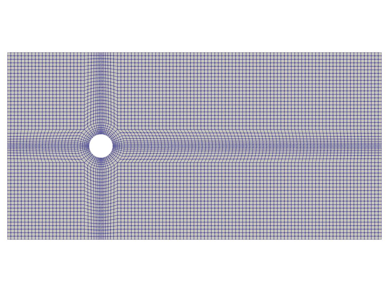
The resulting mesh has fine resolution in the area of interest and has decent non-orthogonality (around 40 degrees).

Checking geometry...
    Overall domain bounding box (-4 -4 -0.01) (12 4 0.01)
    Mesh has 2 geometric (non-empty/wedge) directions (1 1 0)
    Mesh has 2 solution (non-empty) directions (1 1 0)
    All edges aligned with or perpendicular to non-empty directions.
    Boundary openness (-6.7961e-19 3.04482e-18 -1.66941e-13) OK.
    Max cell openness = 4.34617e-16 OK.
    Max aspect ratio = 9.60439 OK.
    Minimum face area = 2.52457e-06. Maximum face area = 0.000632222.  Face area magnitudes OK.
    Min volume = 5.04914e-08. Max volume = 1.26444e-05.  Total volume = 2.54429.  Cell volumes OK.
    Mesh non-orthogonality Max: 44.1274 average: 7.02609
    Non-orthogonality check OK.
    Face pyramids OK.
    Max skewness = 0.433471 OK.
    Coupled point location match (average 0) OK.

Schemes, linear solvers, convergence, and time step controls

Discretization schemes are configured in the fvSchemes file in the system sub-folder of the case. Because the mesh inhibits non-orthogonality, we use the leastSquares gradient reconstruction scheme. The second-order upwind scheme is used for the convection term, and linear corrected schemes are used for the Laplacian and interpolation.

gradSchemes
{
    default         leastSquares;
}


divSchemes
{
    default         none;
    div(phi,U)      Gauss linearUpwind grad(U);

    div((nuEff*dev2(T(grad(U))))) Gauss linear;
}

For the pimpleFoam solver, we need two sets of linear solvers: one for the outer iterations before convergence and the other for the final iteration, which is performed after the convergence is reached.

For the pressure, we use the Geometric Algebraic Multi-Grid (GAMG) solver. Linear solver convergence is controlled by two tolerances: relative and absolute. The first is a measure of the residual reduction; in our case, if the initial residual of the pressure equation is reduced 10 times, we assume that the solver is converged. For the final iteration, we switch to the Preconditioned Conjugate Gradient (PCG) solver with GAMG as a preconditioner. This time we set relative tolerance to 0, so we use absolute tolerance as a convergence criterion for the linear system solver. GAMG uses mesh coarsening to solve a smaller linear system and then propagates the solution on the dense mesh. Since our mesh is static, we can cache agglomeration using cacheAgglomeration flag.

p
{
    solver          GAMG;
    smoother        GaussSeidel;
    tolerance       1E-8;
    relTol          0.1;
    cacheAgglomeration true;
}


pFinal
{
    solver          PCG;
    preconditioner
    {
        preconditioner  GAMG;
        smoother        GaussSeidel;
        tolerance       1E-8;
        relTol          1E-2;
        cacheAgglomeration true;
    }
    tolerance       1E-8;
    relTol          0;
}

Usage of the relative tolerance during initial convergence could accelerate the solution. As we do pressure-velocity coupling, we do not use small tolerances either for the pressure or for the velocity field, since both fields are just an intermediate solution. As we have converged to a solution, we use absolute tolerance to ensure a well-converged solution.

To control the solution convergence residualControl sub-dictionary of the PIMPLE dictionary is used. There we provide field names, relative tolerance, and absolute tolerance.

residualControl
{
    "(U|p)"
    {
        relTol 0;
        tolerance 1e-6;
    }
}

On each outer iteration, the solver checks the initial residual of the linear system for each configured field (in our case, we used a regular expression to match velocity and pressure fields, but they can be configured in separate sub-dictionaries). If the initial residual of the system goes below absolute tolerance or the ratio between current and initial residuals goes below relative tolerance, we assume that the solution has converged.

Simulation stability depends on the time step value. One way to keep the simulation stable is to use a constant small time step. But it is painfully slow, so it is much more convenient to have the time step adapted to the flow field. For the purpose pimpleFoam has the following settings in the controlDict file:

adjustTimeStep yes;

maxCo 0.5;

A rather conservative value of 0.5 for the maximum Courant number is chosen since we use second-order discretization schemes; with the upwind we can use larger value.

Run-time post-processing

We need not only to calculate the flow field but also to extract certain data from the simulation. This is achieved through the run-time post-processing with the function objects. They are configured in the functions sub-dictionary in the controlDict file. To simplify management of the function objects, each description is moved to a separate file; all of them are then included in the corresponding sub-dictionary.

functions
{
    #include "<case>/system/forceCoeffs"
    #include "<case>/system/surfaces"
    #include "<case>/system/timeInfo"
}

Force coefficients

forces
{
    type            forceCoeffs;
    libs            (forces);
    writeControl    adjustableRunTime;
    writeInterval   0.1;

    patches         (cylinder);
    rho             rhoInf;
    log             true;
    rhoInf          1;
    liftDir         (0 1 0);
    dragDir         (1 0 0);
    CofR            (0 0 0);
    pitchAxis       (0 0 1);
    magUInf         $Uin;
    lRef            $D;
    Aref            #eval "2*$dz*$D";
}

To compare the results of the simulations with the experimental data, we need to extract drag and lift forces acting on the cylinder. For this purpose, we use the forceCoeffs function object. Configuration specific to the function object starts from the patches keyword. We configure the patches, which are affected by the forces (in this case, it is a cylinder boundary patch). We set the density of the fluid with the rho keyword. As our simulation is incompressible, we use constant rhoInf as the density. For the calculation of the forces, we need to define drag and lift directions, center of rotation, pitch axis, freestream velocity, reference length scale, and reference area. In our case, drag direction is X, lift direction is Y, and the center of rotation is the center of the cylinder, pitch axis direction is Z, and freestream velocity is the inlet velocity. The reference length scale is the cylinder diameter, and the reference area is the reference length scale multiplied by the thickness of the mesh in the Z direction.

The function object writes in the file postProcessing/forces/0/coefficients.dat values of the coefficients (drag (Cd), lift (Cl), side-force (Cs), and roll (CmRoll), pitch (CmPitch), and yaw (CmYaw) moments). The function object also outputs the coefficients in terms of their front and rear axle constituents ((f) and (r) suffixes).

Sampling

velocity
{
    type            surfaces;
    libs            (sampling);
    writeControl    writeTime;
    surfaceFormat   raw;

    fields
    (
        U
    );

    interpolationScheme cellPoint;

    surfaces
    {
        centerPlane
        {
            type        cuttingPlane;
            point       (0 0 0);
            normal      (0 0 1);
            interpolate true;
            triangulate true;
        }
    }
}

We also extract velocity values along the center plane of the channel. The cuttingPlane function object is used for the purpose. The function object can output the sampled data in different formats; for plotting, we have chosen VTK as the cylinder is a hole in the data, and it needs to be correctly triangulated.

Solver performance information

timeInfo
{
    type            timeInfo;
    libs            (utilityFunctionObjects);
    perTimeStep     yes;
    writeControl    timeStep;
    writeInterval   1;
}

To have a bit of data on the solver performance, we use the timeInfo function object. For each time step, it outputs the current time, total CPU time used, total wall clock time used, CPU time per time step, and wall clock time per time step. Clock time has a resolution of 1 second, so it is not quite useful.

Results

To add a benchmark nature to the simulations, we have decided to compare different OpenFOAM version outputs. There are v2306, v2312, v2412, and v2606 versions installed on the cluster, so the simulations were executed with all these versions and with different mesh sizes: 5k, 30k, and 300k cells.

Dependence of the output on the mesh density is compared for version v2606. Performance of the solver is compared for different versions of OpenFOAM.

Drag and lift coefficient

Good news: all tested OpenFOAM versions calculate the same value for the drag and lift coefficients:

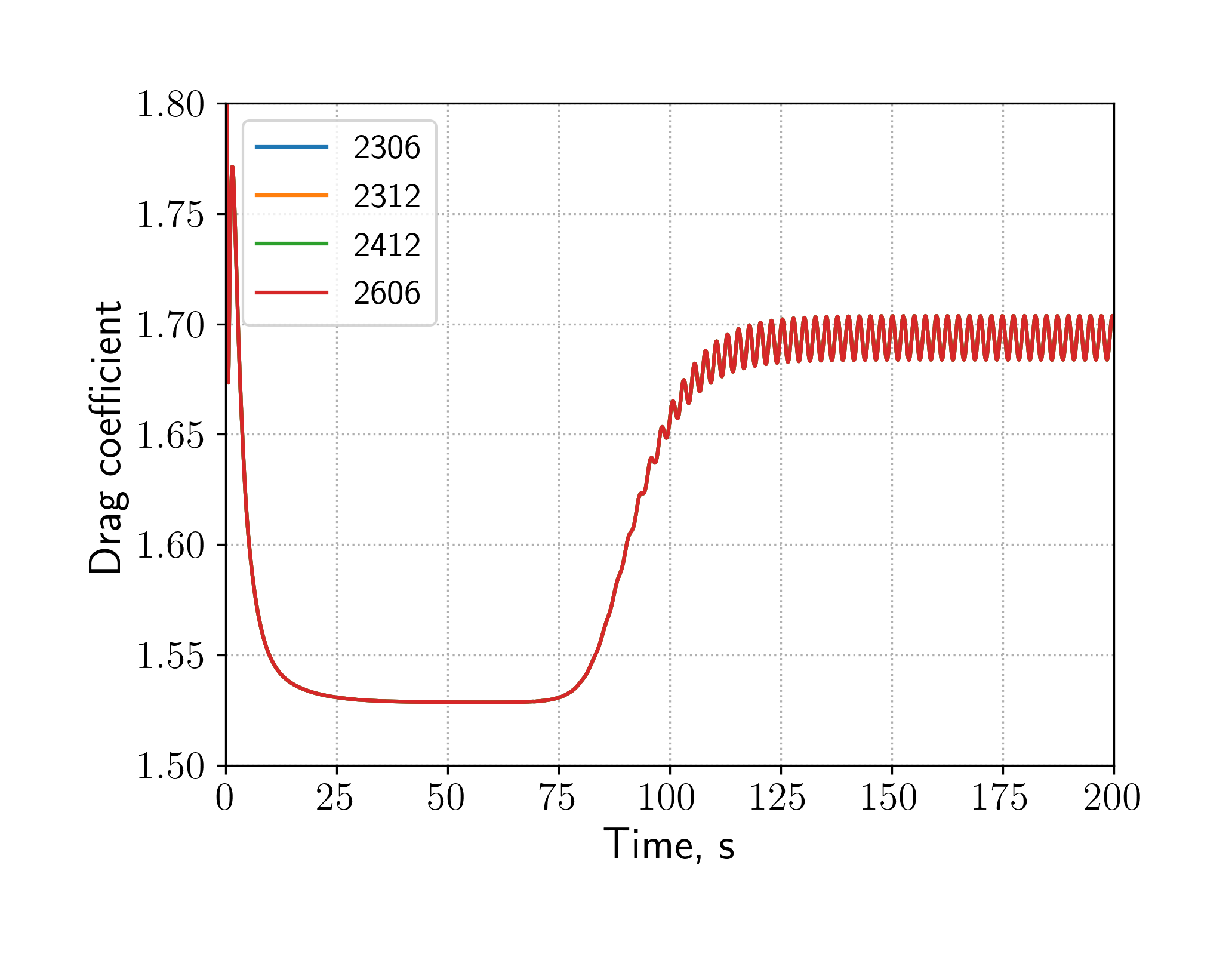
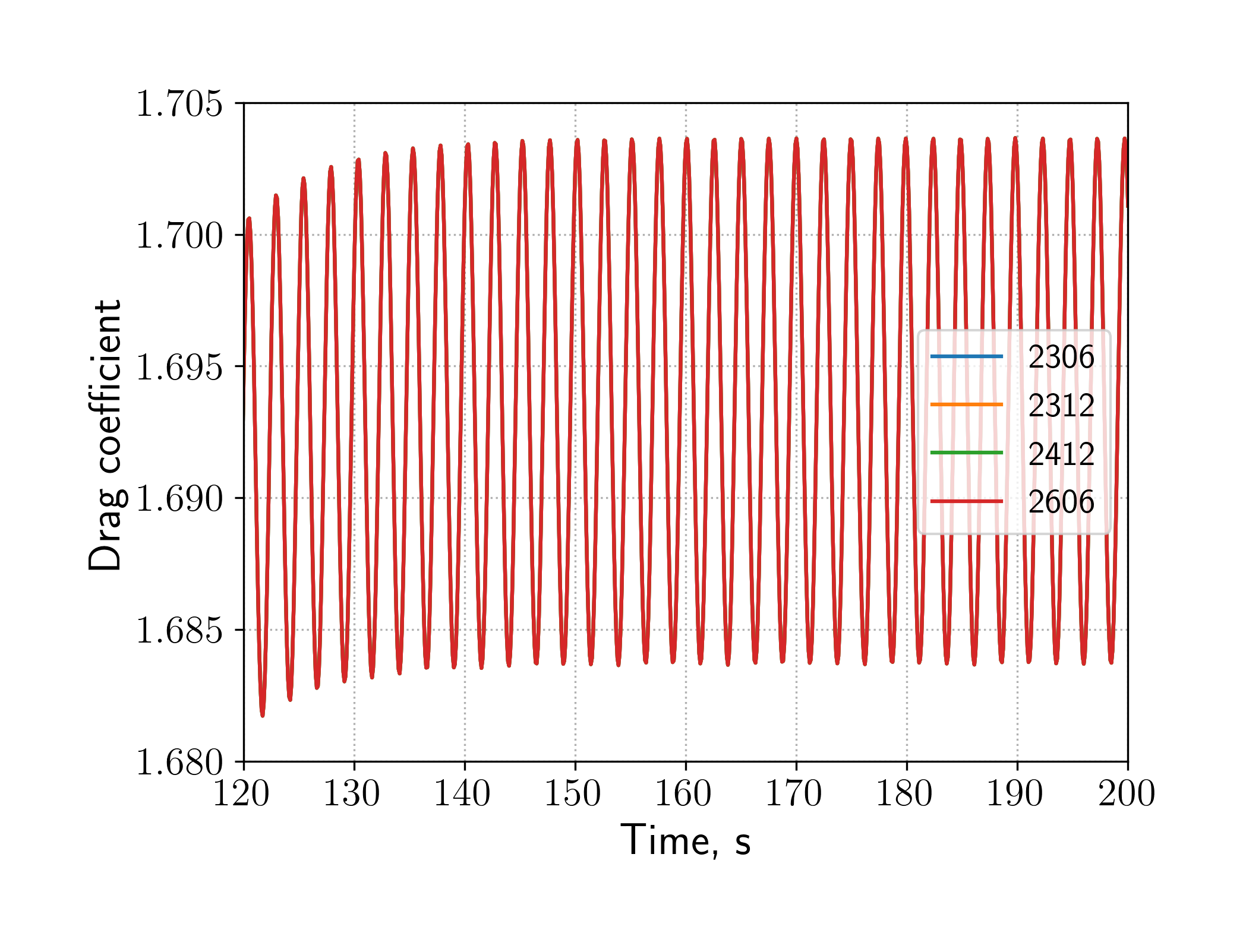
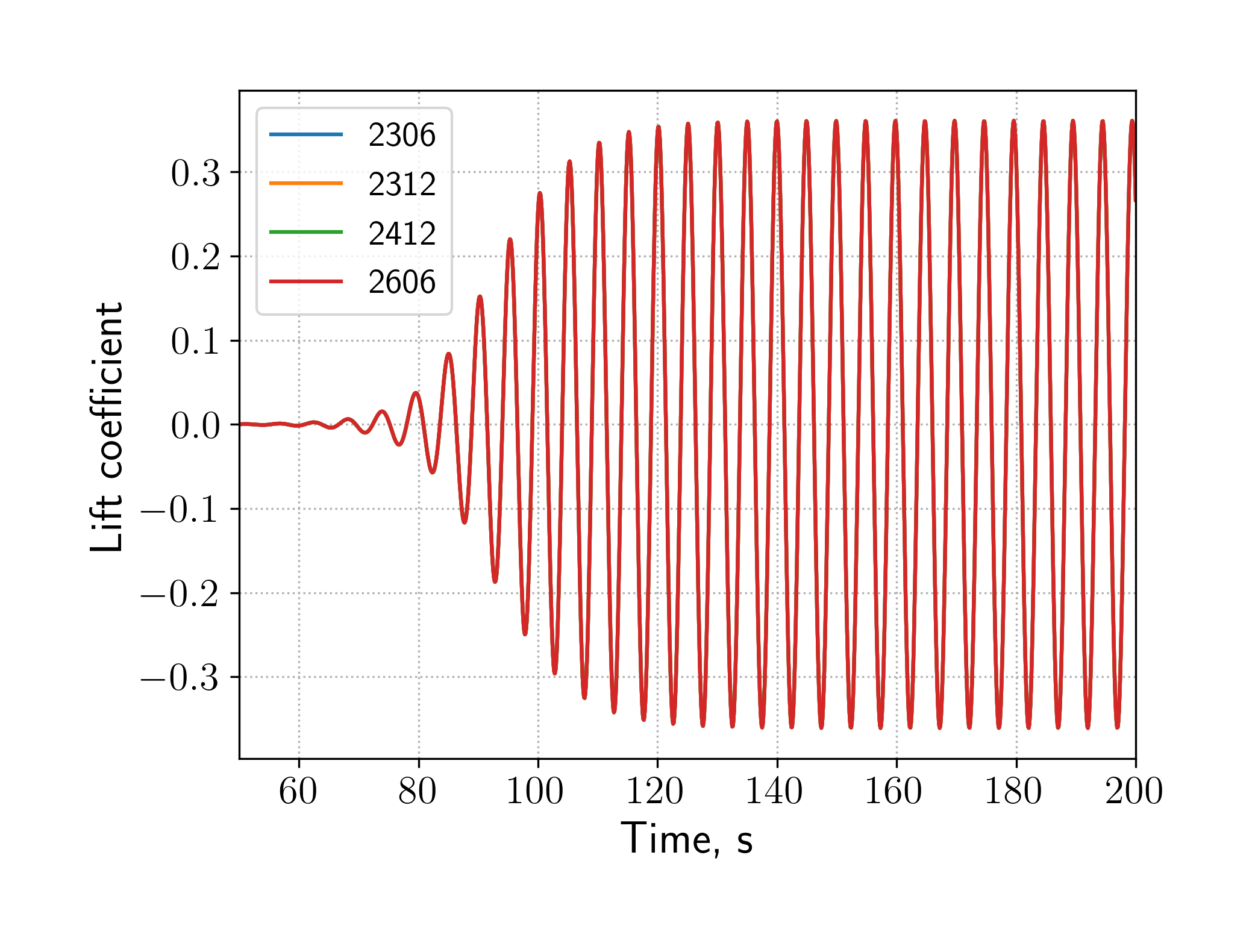
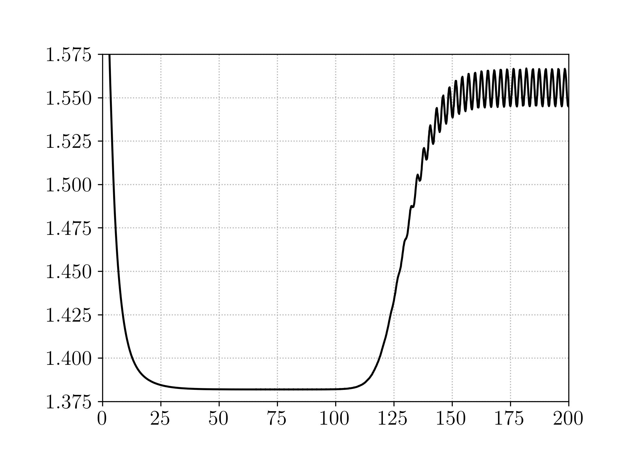
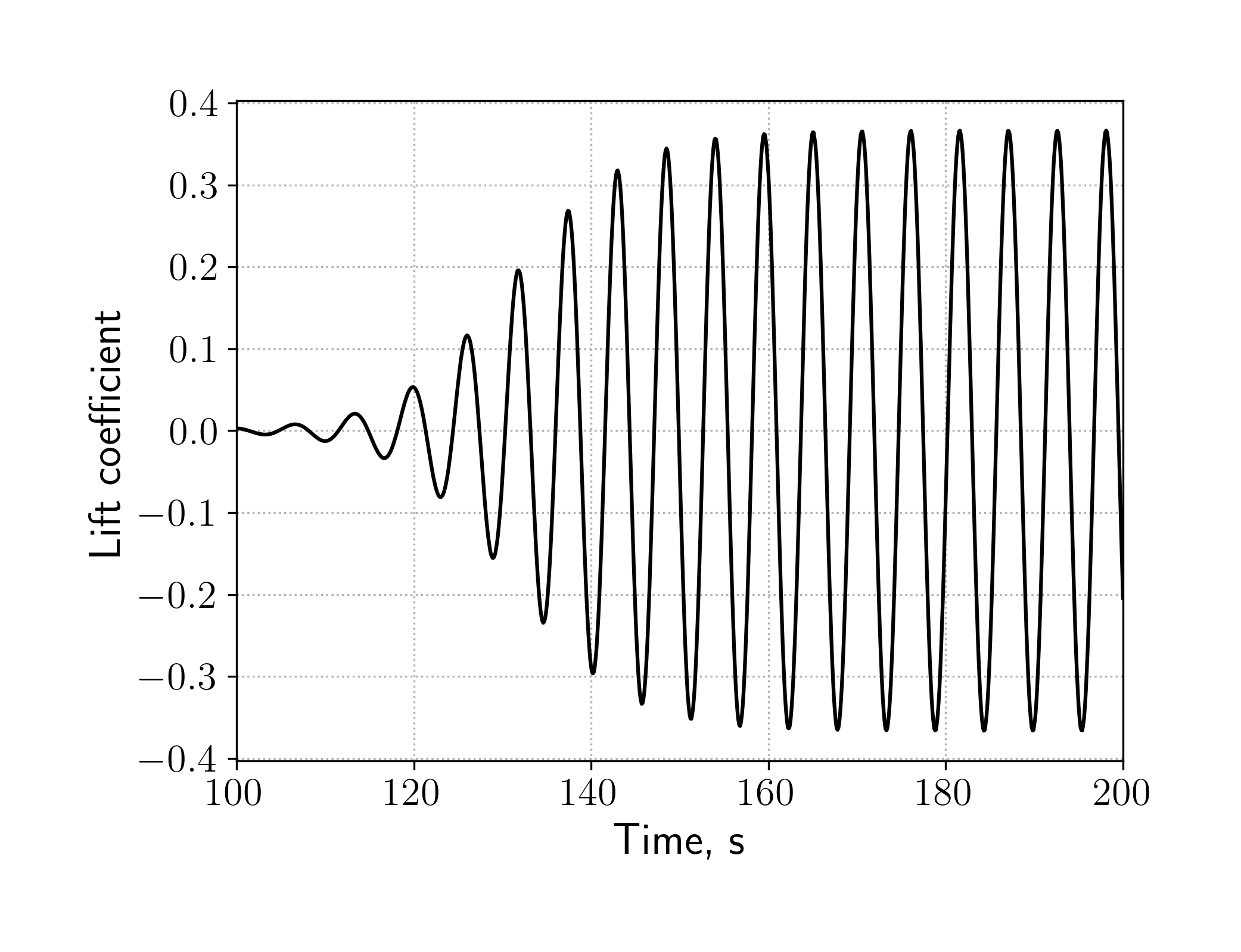
The difference in the drag and lift coefficient values from the cited article is mainly caused by the different boundary conditions on the channel walls. If we make channel walls symmetry planes instead (effectively simulating an array of cylinders, like in the article), values of Cd and Cl become closer to the published ones.

Solver performance

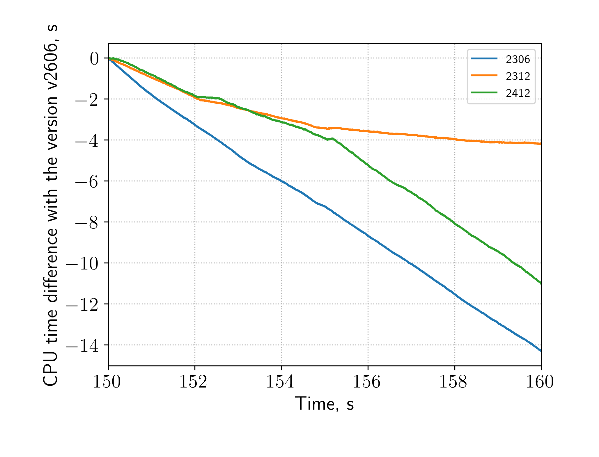
To compare the solver performance difference between versions, the solver was run from a point of 150 s to 160 s with a constant time step (0.002 s) on a 30k-cell mesh.

CPU time for the version v2606 was chosen as a base, and the difference in CPU time was plotted. And it turned out that version v2606 is the slowest. The fastest is v2306, which was 14 seconds faster than v2606. The whole simulation took 1157 seconds of CPU time, so v2306 is 1% faster. This can be attributed to the measurement technique and may be ignored.

Case files

The case files can be found in the show cases repository:

https://code.o2m.solutions/o2m/show-cases/src/branch/trunk/von-karman-vortex-street